Graphene on SiO2 (alpha-quartz): Doping and Gap at the Dirac Point

1. Introduction

This tutorial calculates the band structure of the graphene on O-terminated α-quartz(0001) interface created in the structure tutorial, then reads the position of the Dirac point relative to the Fermi level and the gap at K, reproducing results from the following manuscript. The calculation uses density functional theory (DFT) in the local density approximation (LDA) with GBRV (Garrity-Bennett-Rabe-Vanderbilt) ultrasoft pseudopotentials; a self-consistent field (SCF) step precedes the band path.

Manuscript

Yong-Ju Kang, Joongoo Kang, and K. J. Chang Electronic structure of graphene and doping effect on SiO2 Physical Review B 78, 115404 (2008) DOI: 10.1103/PhysRevB.78.115404 ¹

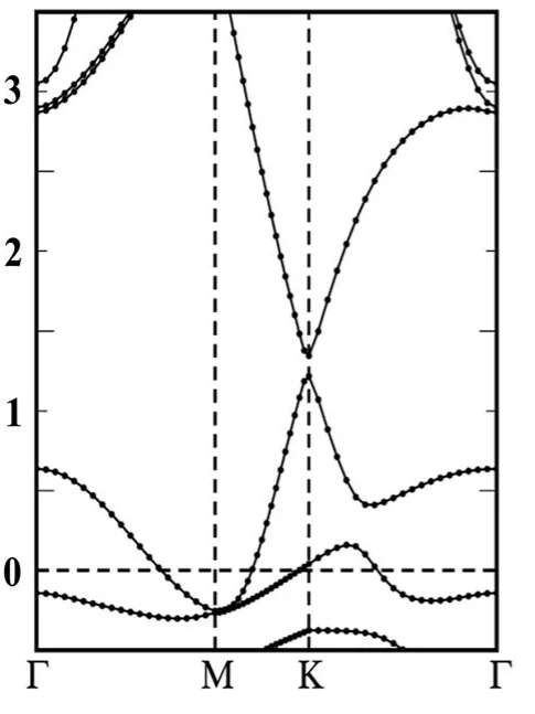
The compared quantities are from Sec. III and Fig. 3(a) of the manuscript, for the metastable geometry with the graphene at d = 2.58 Å above the surface: graphene is p-doped, the gap at the Dirac point is 0.13 eV, and the Dirac point lies about 1.28 eV above the Fermi level (the midpoint of the two Dirac bands at K on Fig. 3(a), +1.21 and +1.35 eV).

2. Prerequisites

Run the structure creation tutorial first. Its interface_2d_3d_graphene_silicon_dioxide.ipynb notebook saves the interface in the 120° setting to the uploads folder under the name C(001)-O2Si(001), Interface, Strain 1.875pct, which this notebook loads. It also shifts graphene to the metastable registry and centers the slab along z. An interface from the generic ZSL notebook comes out at 60°, where the band path's K is not graphene's K.

3. Workflow overview

The notebook runs the Standata band_structure.json workflow, which chains pw_scf and pw_bands, as one job on the interface. With RELAX = True, add_relaxation() puts a relaxation (fixed cell, the pw_vc-relax unit with calculation = 'relax', the same k-mesh as the SCF) in front of it in the same job, and the band structure runs on the relaxed structure.

The notebook then reads the band structure at K, takes the Dirac point as the midpoint of the Dirac pair of bands, and prints it and the gap beside the manuscript's values. Re-running the notebook finds an already-finished job by its material and workflow name and reuses it instead of resubmitting.

4. Calculation parameters

Cell 1.2 sets the material name:

# Name saved by interface_2d_3d_graphene_silicon_dioxide.ipynb.
INTERFACE_NAME = "C(001)-O2Si(001), Interface, Strain 1.875pct"

Cell 1.3 sets the organization, the cluster and the workflow names:

from datetime import datetime
from mat3ra.ide.compute import QueueName

ORGANIZATION_NAME = None  # set to your organization name (full or partial); otherwise, your default one is used
FOLDER = "./uploads"

BAND_STRUCTURE_WORKFLOW_SEARCH_TERM = "band_structure.json"
MY_WORKFLOW_NAME = "Band Structure"
APPLICATION_NAME = "espresso"

# NOTE: False reads the band structure of the structure as built: E_D - E_F +1.171 eV, gap at K
# 0.062 eV, about 1 h on OR/16. True relaxes all atoms at fixed cell to 0.03 eV/Å (Kang et al.
# Sec. II) before the band structure, in the same job; on OR/16 it did 5 BFGS steps in the 4 h
# TIME_LIMIT with the force still falling (job 25yp4K2SMNJgJMmBy).
RELAX = False

CLUSTER_NAME = "001"  # specify full or partial name i.e. "cluster-001" to select
QUEUE_NAME = QueueName.OR
PPN = 16  # queue OR on cluster-001 allows at most 16 cores per node
TIME_LIMIT = "04:00:00"

timestamp = datetime.now().strftime("%Y-%m-%d %H:%M")
POLL_INTERVAL = 60  # seconds

Cell 1.4 sets the DFT parameters:

MODEL_SUBTYPE = "lda"
FUNCTIONAL = "pz"  # Kang et al. 2008 use LDA
PSEUDOPOTENTIAL_TYPE = "us"  # GBRV ultrasoft, the only LDA family the platform publishes for Si, O and C
GBRV_VALENCE = {"Si": 4, "O": 6, "C": 4}  # valence electrons per atom of the GBRV pseudopotentials
ECUTWFC = 40   # Ry, GBRV's recommended wavefunction cutoff
ECUTRHO = 200  # Ry, GBRV's recommended charge-density cutoff

KPOINT_DENSITY = 4  # gives 6 x 6 x 1 on the 1x1 quartz cell, Kang et al. Sec. II
SMEARING_SETTINGS = {"degauss": 0.01}  # Ry; the doped graphene has no gap at E_F
KPATH_STEPS = 20
MODEL_TAG = (f"{FUNCTIONAL}-{PSEUDOPOTENTIAL_TYPE} {ECUTWFC}-{ECUTRHO}Ry k{KPOINT_DENSITY} "
             f"p{KPATH_STEPS} g{SMEARING_SETTINGS['degauss']}")

SCF_UNIT = "pw_scf"
BANDS_UNIT = "pw_bands"
RELAX_UNIT = "pw_vc-relax"
# Fixed cell, 0.03 eV/Å, Kang et al. 2008 Sec. II
RELAXATION_SETTINGS = {"calculation": "relax", "forc_conv_thr": 1.17e-3, "nstep": 100}
WORKFLOW_TAG = MODEL_TAG + (f" relax f{RELAXATION_SETTINGS['forc_conv_thr']}" if RELAX else "")

KPATH = [
    {"point": "K", "steps": KPATH_STEPS},
    {"point": "Γ", "steps": KPATH_STEPS},
    {"point": "M", "steps": KPATH_STEPS},
    {"point": "K", "steps": 1},
]
K_INDEX = 0  # KPATH starts at K, so the first point of the band structure's path is K

manuscript	this notebook
LDA	LDA (pz)
ultrasoft pseudopotentials, VASP, 396 eV cutoff (Sec. II)	GBRV ultrasoft, 40/200 Ry
6×6×1 k-mesh, 1×1 quartz cell (Sec. II)	KPOINT_DENSITY = 4, 6×6×1
2×2 graphene on 1×1 quartz	the same, as built by the structure notebook, graphene strained +1.875 %
14 SiO2 bilayers, H-passivated back side	15 Si planes (5 conventional cells; one bilayer read as one Si plane with its O), bare back side
20 Å vacuum	about 20 Å, as built by the structure notebook
manuscript quartz cell	standata quartz cell, 2.3 % larger in a
d = 2.58 Å, metastable geometry (Sec. III)	d = 2.58 Å, graphene shifted in-plane to the metastable registry (REGISTRY_SHIFT in the structure notebook); surface O at 0.354 Å and 1.095 Å from the nearest C

The structure is the example as the structure notebook builds it. The bare back surface is the face the manuscript (p. 2) calls chemically inactive. The structure notebook's cell 3.6 sets the cell to the 120° hexagonal setting and types it HEX, so the symbolic K point of KPATH lies on the band path.

5. Step-by-step instructions

5.1. Open the notebook

Navigate to the API examples repository and open:

other/materials_designer/specific_examples/interface_2d_3d_graphene_silicon_dioxide_SIMULATION.ipynb

5.2. Configure parameters

In cell 1.3, set ORGANIZATION_NAME and CLUSTER_NAME to the account's organization and cluster. INTERFACE_NAME in cell 1.2 already holds the name the structure notebook saves; leave it unchanged unless the material was renamed.

5.3. Run the notebook

Select Run > Run All. The notebook authenticates with the platform, loads the interface and prints its provenance (composition, number of atoms, gamma, interlayer distance of 2.580 Å, valence electrons, occupied bands), configures the DFT model and the k-grid, creates the compute configuration, saves the material to the account, then submits the band structure job and waits for it to finish. For the example as built the provenance reads Si15O30C8, 53 atoms, gamma = 120.000°, 272 valence electrons and 136 occupied bands. Once finished (measured with RELAX = False on cluster-001, queue OR with 16 cores, called OR/16 below: about 1 h), the notebook retrieves the band structure, prints the bands at K around the Fermi level and the Dirac pair, then E_F, E_D − E_F and the gap at K, and prints the comparison with the manuscript.

5.4. Relax the interface (optional)

Set RELAX = True in cell 1.3 and run the notebook. The relaxation (all atoms, fixed cell, force threshold 0.03 eV/Å, Sec. II) runs in the same job before the band structure, and the band structure is taken on the relaxed structure. On OR/16 it did 5 BFGS steps in the 4 h TIME_LIMIT with the force still falling (job 25yp4K2SMNJgJMmBy).

5.5. Re-run the notebook

Running the notebook again finds the finished job by material and workflow name and reuses it rather than resubmitting.

6. Expected results

quantity	manuscript	this notebook, RELAX = False
doping	p-type (Sec. III)	p-type
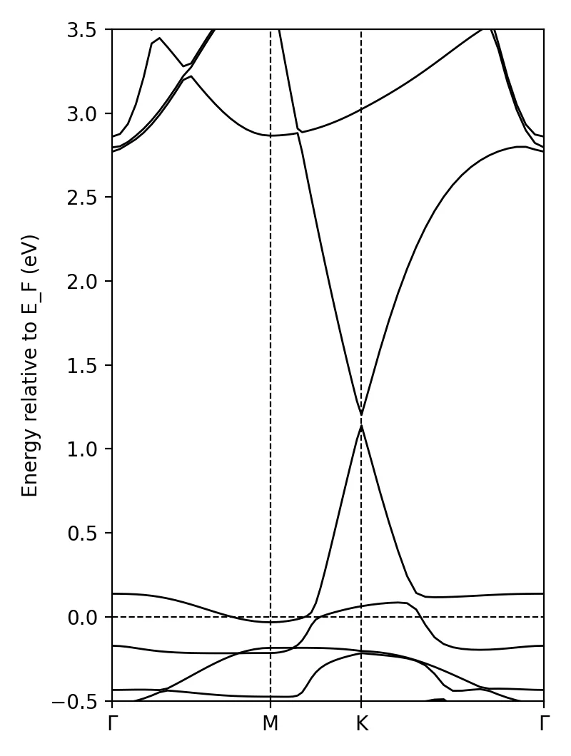
E_D − E_F (eV)	+1.28 (midpoint of the two Dirac bands at K on Fig. 3(a), +1.21 and +1.35 eV)	+1.171
gap at K (eV)	0.13 (Sec. III)	0.062

Kang's gap is for the relaxed metastable geometry (Sec. III); the values above are for RELAX = False on the shifted registry (job F6AmKDRpQ6nFqiokb, unrelaxed, about 1 h on OR/16). The relaxed regime did not converge within the 4 h limit (5 BFGS steps on OR/16). The notebook's final cell prints:

Regime: unrelaxed SCF
                 this notebook    Kang et al. (2008)
Doping                  p-type                p-type
E_D - E_F             1.171 eV              1.280 eV
Gap at K              0.062 eV              0.130 eV

The band structure of the structure after 5 BFGS steps of the RELAX = True relaxation (job domjmuR4659Rj8np5) is p-type, E_D − E_F +1.179 eV, gap at K 0.071 eV, beside the unrelaxed +1.171 eV and 0.062 eV.

7. Customization options

Changing ECUTWFC, ECUTRHO, KPOINT_DENSITY, KPATH_STEPS, SMEARING_SETTINGS["degauss"], RELAX or RELAXATION_SETTINGS["forc_conv_thr"] changes the workflow name, so a new job is created rather than the finished one reused.

8. Troubleshooting

8.1. Material not found

ValueError: No material named … means the structure notebook has not been run, or INTERFACE_NAME does not match. Run the structure tutorial first; the name must be exactly C(001)-O2Si(001), Interface, Strain 1.875pct.

9. Interactive JupyterLite notebook

⛶ Full Screen

10. References

---

1. Yong-Ju Kang, Joongoo Kang, and K. J. Chang. Electronic structure of graphene and doping effect on sio2. Physical Review B, 78:115404, 2008. URL: https://link.aps.org/doi/10.1103/PhysRevB.78.115404. ↩